Google Sheets Tutorial
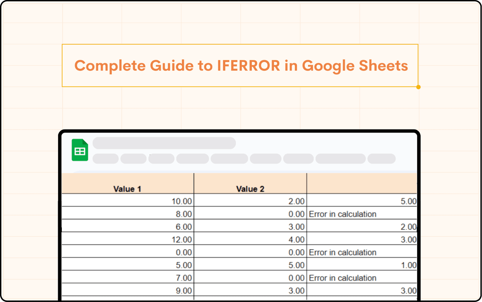
Complete Guide to IFERROR in Google Sheets
Master the IFERROR function in Google Sheets. Learn how to manage and prevent errors in your formulas, ensuring clean, professional, and reliable spreadsheets.
Table of Contents
Google Sheets has become an essential tool for anyone working with data. From business professionals to students, the ease of use and functionality it provides are unmatched. One of its most useful functions, particularly when dealing with large datasets, is the IFERROR function. Understanding how to leverage IFERROR in Google Sheets can save time and reduce errors in your data analysis, ensuring that your results are accurate and your formulas do not break due to unexpected errors.
The IFERROR function will be discussed in this guide together with its significance, how to use it, and numerous efficient approaches of implementation. Whether your experience with Google Sheets is fresh or seasoned, you will find useful advice to improve your spreadsheets abilities.
What is the IFERROR Function?
The IFERROR function in Google Sheets is a powerful tool that helps you manage errors in your formulas. It allows you to replace error messages, such as #DIV/0!, #N/A, or #VALUE!, with a custom message or alternative value. This ensures that your spreadsheet looks cleaner and that your workflow isn't disrupted by errors.
Why Use IFERROR in Google Sheets?
Errors in a spreadsheet can be problematic for several reasons. They can cause formulas to stop working, make data analysis difficult, and create a less professional appearance. By using IFERROR in Google Sheets, you can:
Prevent Disruptions: Ensure that errors don’t cause your formulas to break.
Maintain Data Integrity: Replace errors with a default value that keeps your data consistent.
Enhance User Experience: Provide clear, understandable messages instead of confusing error codes.
Using Superjoin - AI Copilot for Google Sheets
This guide will walk you through the process of using Superjoin to effortlessly use IFERROR in your Google Sheets, saving you time and reducing errors
Step-by-Step Guide:
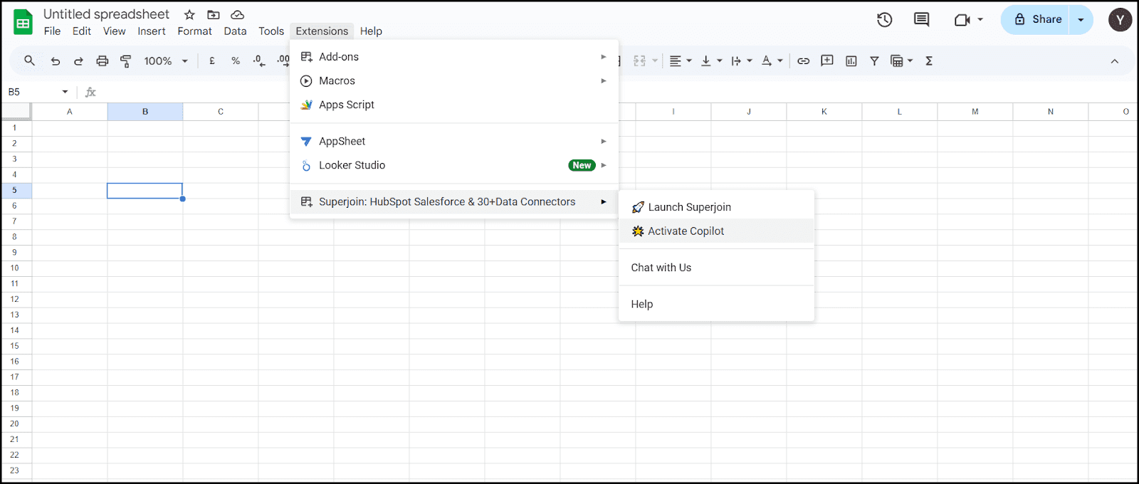
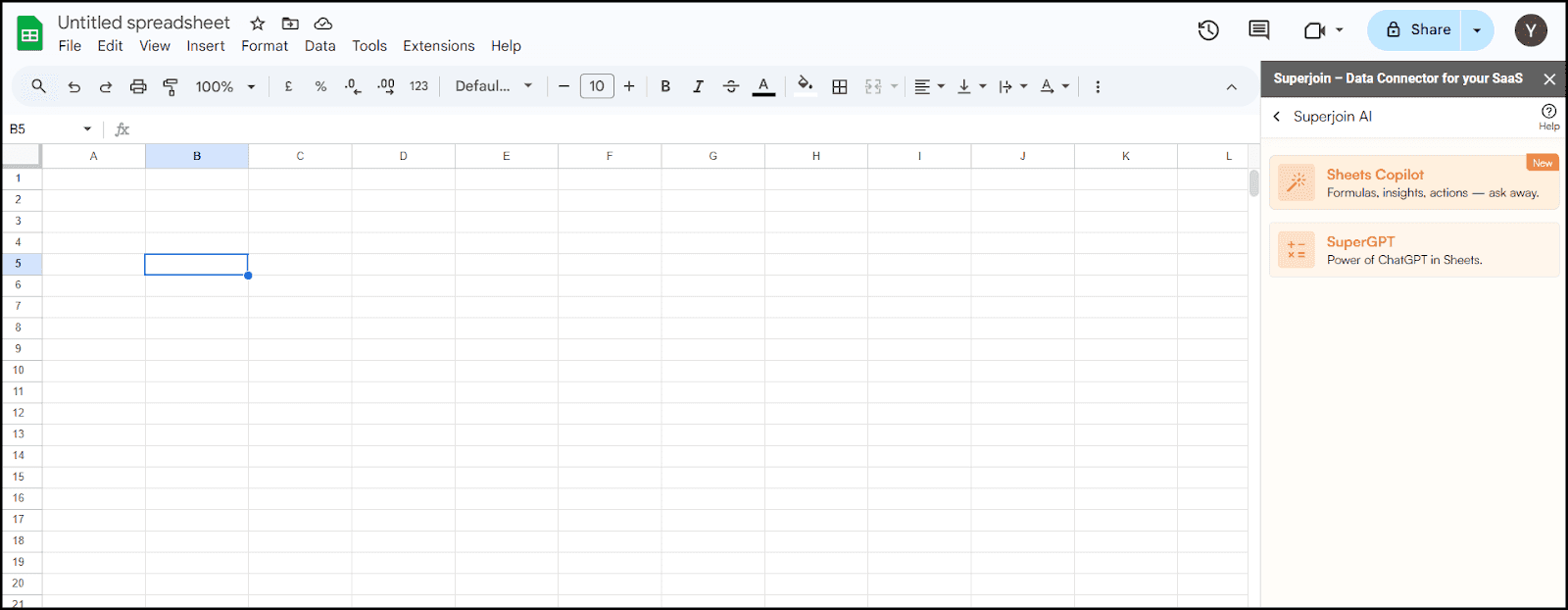
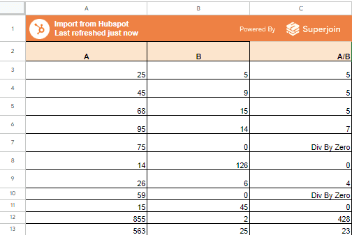
Launch Superjoin: Install the free Superjoin Extension. After installing the extension, navigate to the "Extensions" menu in your Google Sheet. Click on Activate Copilot.
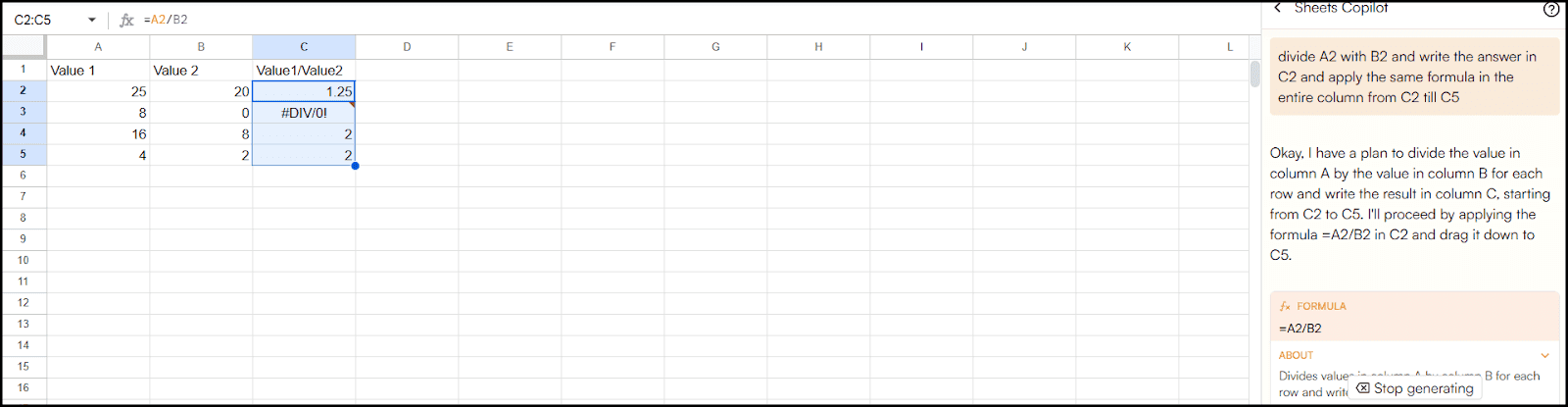
Write the Action Prompt: Use this prompt
divide A2 with B2 and write the answer in C2 and apply the same formula in the entire column from C2 till C5
You can write in simple English what you would like to do.

Execute: Click Enter to start the process. You will see a summary of what Superjoin AI Copilot will be doing. If this is what you expect, accept the solution.
How to Use IFERROR in Google Sheets
Using the IFERROR function is straightforward. Here's the syntax:
=IFERROR(value, [value_if_error])Value: The formula or expression you want to check for errors.
Value_if_error: The value or message you want to display if an error is found.
For example, suppose you have the following formula in cell A2: =B2/C2. If C2 is zero, the formula will return #DIV/0!. To prevent this, you can wrap the formula in IFERROR like this:
=IFERROR(B2/C2, "Div By Zero")
Now, instead of showing #DIV/0!, the cell will display "Div By Zero."
Alternative Methods to Use IFERROR in Google Sheets
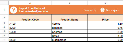
Using IFERROR with Other Functions (VLOOKUP Example)
Dataset:
Steps:
Input Data: Create a dataset in Google Sheets with the columns as shown above (Product Code, Product Name, Price).
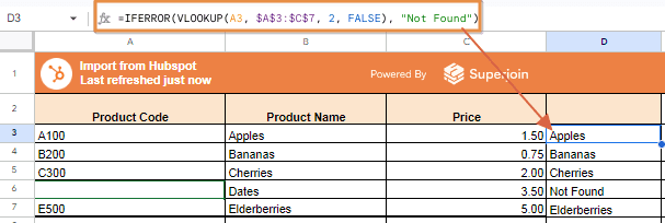
VLOOKUP Formula: In a new cell, try to search for a product using VLOOKUP. For example, enter a product code in cell A2 and use the following formula:
=VLOOKUP(A2, B2:C10, 2, FALSE)
If the product code is not found, it will return #N/A.
Apply IFERROR: Modify the VLOOKUP formula to handle errors with IFERROR:
=IFERROR(VLOOKUP(A3, $A$3:$C$7, 2, FALSE), "Not Found")Now, if the product code is not found, it will return "Not Found" instead of #N/A.
Handling Multiple Errors with Nested IFERROR
Sometimes, a formula may produce different types of errors, and you might want to handle each one differently. By nesting IFERROR functions, you can achieve this. Here's an example:
Dataset:
Steps:
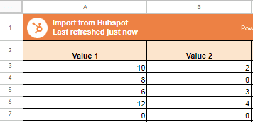
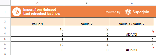
Input Data: Create a dataset in Google Sheets with the columns as shown above (Value 1 and Value 2).
Division Formula: In a new cell, divide the two values using a simple formula like A2/B2. For example:
=A2/B2
This may return errors such as #DIV/0! if B2 is zero.
Apply Nested IFERROR: Use IFERROR to handle different types of errors. Here’s an example formula:
=IFERROR(A2/B2, IFERROR(A2/B2, "Another Error"))
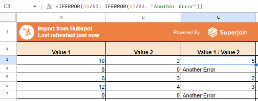
In this example, the formula will first check for an error in the division, and if found, will replace it with the custom error message "Another Error".
Using Array Formulas with IFERROR
Array formulas in Google Sheets allow you to perform operations on a range of cells. Combining IFERROR with array formulas can streamline error handling across multiple cells.
Dataset:
Steps:
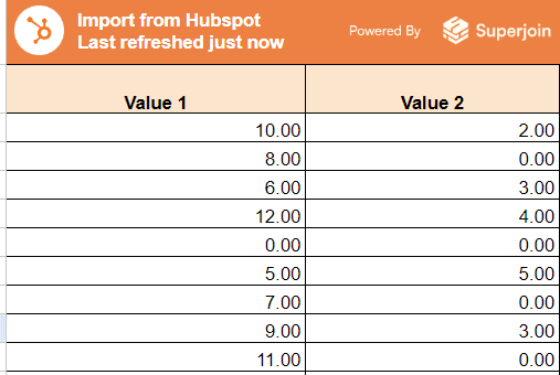
Input Data: Create a dataset in Google Sheets with the columns as shown above (Value 1 and Value 2).
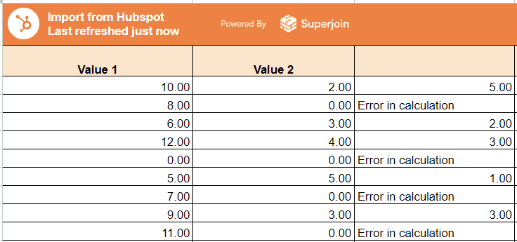
Apply Division Across a Range: Use an ARRAYFORMULA to perform division across a range. For example:
=ARRAYFORMULA(A3:A11/B3:B11)
This will apply the division to each corresponding row in the ranges A3:A11 and B3:B11.
Combine with IFERROR: Add IFERROR to handle any errors that occur during the division:
=ARRAYFORMULA(IFERROR(A3:A11/B3:B11, "Error in calculation"))
Now, any division that results in an error (like dividing by zero) will return "Error in calculation".
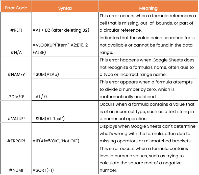
Types of Google Sheets Errors — And Their Importance
The IFERROR function in Google Sheets is designed to return a specified value when a formula encounters a parse error. A parse error occurs when Google Sheets is unable to understand or execute a formula.
In Google Sheets, parse errors are formal entities that function like IFERROR can handle. These errors can result from typos, impossible mathematical operations, or other issues that disrupt a formula's execution.
To effectively use the IFERROR function, it's essential to understand the different types of errors and what they signify. Below are the common error codes that Google Sheets may return:
Best Practices for Using IFERROR in Google Sheets
Use Meaningful Messages: Instead of a generic "Error," provide context-specific messages that help users understand what went wrong.
Apply IFERROR Judiciously: Overusing IFERROR can mask underlying issues in your data. Use it strategically where errors are expected or manageable.
Combine with Other Error-Handling Techniques: In complex spreadsheets, consider combining IFERROR with data validation rules, conditional formatting, and other error-handling strategies.
Conclusion
Understanding and applying IFERROR in Google Sheets is essential for anyone who regularly works with spreadsheets. This function not only helps you manage and prevent errors but also enhances the overall user experience by keeping your data clean and professional. By integrating IFERROR with other Google Sheets functions and adopting best practices, you can take your spreadsheet skills to the next level.
Say Goodbye to Tedious Data Exports! 🚀
Are you tired of the hassle of manually moving data from various tools into Google Sheets? Superjoin has a solution for you.
Superjoin is a Google Sheets add-on that automatically connects your favorite SaaS tools to your spreadsheets. It pulls data directly into Google Sheets, allowing you to create reports that update themselves without any manual work on your part.
Google Sheets has become an essential tool for anyone working with data. From business professionals to students, the ease of use and functionality it provides are unmatched. One of its most useful functions, particularly when dealing with large datasets, is the IFERROR function. Understanding how to leverage IFERROR in Google Sheets can save time and reduce errors in your data analysis, ensuring that your results are accurate and your formulas do not break due to unexpected errors.
The IFERROR function will be discussed in this guide together with its significance, how to use it, and numerous efficient approaches of implementation. Whether your experience with Google Sheets is fresh or seasoned, you will find useful advice to improve your spreadsheets abilities.
What is the IFERROR Function?
The IFERROR function in Google Sheets is a powerful tool that helps you manage errors in your formulas. It allows you to replace error messages, such as #DIV/0!, #N/A, or #VALUE!, with a custom message or alternative value. This ensures that your spreadsheet looks cleaner and that your workflow isn't disrupted by errors.
Why Use IFERROR in Google Sheets?
Errors in a spreadsheet can be problematic for several reasons. They can cause formulas to stop working, make data analysis difficult, and create a less professional appearance. By using IFERROR in Google Sheets, you can:
Prevent Disruptions: Ensure that errors don’t cause your formulas to break.
Maintain Data Integrity: Replace errors with a default value that keeps your data consistent.
Enhance User Experience: Provide clear, understandable messages instead of confusing error codes.
Using Superjoin - AI Copilot for Google Sheets
This guide will walk you through the process of using Superjoin to effortlessly use IFERROR in your Google Sheets, saving you time and reducing errors
Step-by-Step Guide:
Launch Superjoin: Install the free Superjoin Extension. After installing the extension, navigate to the "Extensions" menu in your Google Sheet. Click on Activate Copilot.
Write the Action Prompt: Use this prompt
divide A2 with B2 and write the answer in C2 and apply the same formula in the entire column from C2 till C5
You can write in simple English what you would like to do.
Execute: Click Enter to start the process. You will see a summary of what Superjoin AI Copilot will be doing. If this is what you expect, accept the solution.
How to Use IFERROR in Google Sheets
Using the IFERROR function is straightforward. Here's the syntax:
=IFERROR(value, [value_if_error])Value: The formula or expression you want to check for errors.
Value_if_error: The value or message you want to display if an error is found.
For example, suppose you have the following formula in cell A2: =B2/C2. If C2 is zero, the formula will return #DIV/0!. To prevent this, you can wrap the formula in IFERROR like this:
=IFERROR(B2/C2, "Div By Zero")
Now, instead of showing #DIV/0!, the cell will display "Div By Zero."
Alternative Methods to Use IFERROR in Google Sheets
Using IFERROR with Other Functions (VLOOKUP Example)
Dataset:
Steps:
Input Data: Create a dataset in Google Sheets with the columns as shown above (Product Code, Product Name, Price).
VLOOKUP Formula: In a new cell, try to search for a product using VLOOKUP. For example, enter a product code in cell A2 and use the following formula:
=VLOOKUP(A2, B2:C10, 2, FALSE)
If the product code is not found, it will return #N/A.
Apply IFERROR: Modify the VLOOKUP formula to handle errors with IFERROR:
=IFERROR(VLOOKUP(A3, $A$3:$C$7, 2, FALSE), "Not Found")Now, if the product code is not found, it will return "Not Found" instead of #N/A.
Handling Multiple Errors with Nested IFERROR
Sometimes, a formula may produce different types of errors, and you might want to handle each one differently. By nesting IFERROR functions, you can achieve this. Here's an example:
Dataset:
Steps:
Input Data: Create a dataset in Google Sheets with the columns as shown above (Value 1 and Value 2).
Division Formula: In a new cell, divide the two values using a simple formula like A2/B2. For example:
=A2/B2
This may return errors such as #DIV/0! if B2 is zero.
Apply Nested IFERROR: Use IFERROR to handle different types of errors. Here’s an example formula:
=IFERROR(A2/B2, IFERROR(A2/B2, "Another Error"))
In this example, the formula will first check for an error in the division, and if found, will replace it with the custom error message "Another Error".
Using Array Formulas with IFERROR
Array formulas in Google Sheets allow you to perform operations on a range of cells. Combining IFERROR with array formulas can streamline error handling across multiple cells.
Dataset:
Steps:
Input Data: Create a dataset in Google Sheets with the columns as shown above (Value 1 and Value 2).
Apply Division Across a Range: Use an ARRAYFORMULA to perform division across a range. For example:
=ARRAYFORMULA(A3:A11/B3:B11)
This will apply the division to each corresponding row in the ranges A3:A11 and B3:B11.
Combine with IFERROR: Add IFERROR to handle any errors that occur during the division:
=ARRAYFORMULA(IFERROR(A3:A11/B3:B11, "Error in calculation"))
Now, any division that results in an error (like dividing by zero) will return "Error in calculation".
Types of Google Sheets Errors — And Their Importance
The IFERROR function in Google Sheets is designed to return a specified value when a formula encounters a parse error. A parse error occurs when Google Sheets is unable to understand or execute a formula.
In Google Sheets, parse errors are formal entities that function like IFERROR can handle. These errors can result from typos, impossible mathematical operations, or other issues that disrupt a formula's execution.
To effectively use the IFERROR function, it's essential to understand the different types of errors and what they signify. Below are the common error codes that Google Sheets may return:
Best Practices for Using IFERROR in Google Sheets
Use Meaningful Messages: Instead of a generic "Error," provide context-specific messages that help users understand what went wrong.
Apply IFERROR Judiciously: Overusing IFERROR can mask underlying issues in your data. Use it strategically where errors are expected or manageable.
Combine with Other Error-Handling Techniques: In complex spreadsheets, consider combining IFERROR with data validation rules, conditional formatting, and other error-handling strategies.
Conclusion
Understanding and applying IFERROR in Google Sheets is essential for anyone who regularly works with spreadsheets. This function not only helps you manage and prevent errors but also enhances the overall user experience by keeping your data clean and professional. By integrating IFERROR with other Google Sheets functions and adopting best practices, you can take your spreadsheet skills to the next level.
Say Goodbye to Tedious Data Exports! 🚀
Are you tired of the hassle of manually moving data from various tools into Google Sheets? Superjoin has a solution for you.
Superjoin is a Google Sheets add-on that automatically connects your favorite SaaS tools to your spreadsheets. It pulls data directly into Google Sheets, allowing you to create reports that update themselves without any manual work on your part.
FAQs
Can I use IFERROR with custom formulas in Google Sheets?
Can I use IFERROR with custom formulas in Google Sheets?
How does IFERROR differ from the IF function in Google Sheets?
How does IFERROR differ from the IF function in Google Sheets?
Is there a way to handle multiple errors differently in one formula?
Is there a way to handle multiple errors differently in one formula?
Automatic Data Pulls
Visual Data Preview
Set Alerts
other related blogs
Try it now