Google Sheets Tutorial
Easily Organize Your Data Using Header in Google Sheets
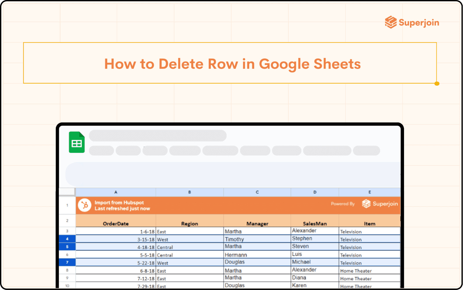
This Article focuses on effectively using Header rows in Google Sheets to organize your data with techniques that make Data Handling easier.


Imagine a cluttered desk overflowing with papers. You know exactly where everything is – that specific report is under the blue stapler, and the client notes are buried beneath a half-eaten granola bar wrapper. But for anyone else trying to navigate this chaos, it's a disaster zone. This is exactly what an unorganized spreadsheet can feel like. Data is scattered, categories are unclear, and finding what you need becomes a frustrating treasure hunt.
The solution? A well-defined header row in Google Sheets. Just like labels on file folders bring order to your physical workspace, a header row acts as a guide for your spreadsheet, making your data crystal clear and readily accessible.
Benefits of Using Header Rows
Think of a header row as the roadmap for your spreadsheet. It offers a multitude of advantages:
Enhanced Readability: Clear labels instantly identify the content in each column, eliminating confusion and saving you time deciphering cryptic data entries.
Efficient Sorting and Filtering: Header rows are the key to unlocking Google Sheets' powerful sorting and filtering functions. Need to see your customer list by last name? Simply sort by the "Last Name" header.
Data Validation: Want to ensure consistency and accuracy in your data entry? Header rows can be used to set up data validation rules, restricting users from entering invalid information.
Improved Collaboration: When multiple people are working on a spreadsheet, a well-defined header row ensures everyone is on the same page and understands the data structure.
How to Freeze the Header Row in Google Sheets
The "Freeze" function is your best friend for keeping your header row visible while scrolling through extensive data sets. This technique is particularly helpful for large spreadsheets.
Here’s how you can freeze a header row in Google Sheets using simple steps:
Step 1: Creating Header Row: Click on the first row (row number 1) and type in the labels for each column.
Step 2: Using Freeze Panes: Click on the row below your desired header row (typically row number 2). Then, navigate to the "View" menu and select "Freeze" followed by "1 row."
This will lock the top row in place, ensuring your headers are always in sight. This allows you to maintain context and easily navigate your spreadsheet, regardless of how far down you've ventured.
Formatting Your Header Row
Now that you have your header row in place, it's time to make it stand out! Here's how to format your header row for optimal clarity and visual appeal:
Bolding and Font Size: Increase the font size and bold the text in your header row to differentiate it from the rest of your data. This will draw the reader's eye and make the headers easy to identify.
Text Alignment and Borders: Align the text in your header row to the center or left for a clean look. Consider adding borders around the header row cells to further define the separation between headers and data.
Background Color and Shading: Using a subtle background color or shading for your header row can further enhance its visual distinction.
Advanced Header Row Techniques
Once you've mastered the basics, Google Sheets offers some advanced techniques to elevate your header row game:
Merging Cells for Combined Headers: For broader categories spanning multiple columns, you can merge cells in your header row to create a single, overarching label.
Filtering Data by Header Row: The magic of header rows truly shines when paired with filtering. Click the filter icon (a downward-facing arrow) next to a header to display a menu for filtering your data based on specific criteria within that column.
Using Drop-Down Lists in Headers: Create a drop-down list in your header row cell to limit data entry to predefined options. This ensures consistency and reduces the risk of errors.
Conditional Formatting Based on Headers: Conditional formatting allows you to apply visual cues based on the data in your spreadsheet. You can leverage your header row to set up rules that highlight specific values or data points within a column.
Tips for Effective Header Rows
Now that you've got the technical aspects down, here are some additional tips to ensure your header rows are truly effective:
Descriptive and Clear Labels: Don't use abbreviations or jargon. Instead, opt for clear and concise labels that accurately reflect the content within each column.
Consistent Capitalization: Maintain consistent capitalization throughout your header row. This may seem like a minor detail, but it contributes to a professional and polished look.
Using Data Validation: Data validation allows you to restrict the type of data that can be entered into specific columns. This can be particularly useful for ensuring consistency in units of measurement, date formats, or other data types.
Conclusion
A well-defined header row forms the foundation of a well-organized and user-friendly spreadsheet. By implementing the techniques discussed above, you can transform your Google Sheets into efficient data management tools that save you time, improve accuracy, and foster seamless collaboration. Remember, a little planning goes a long way, and a well-crafted header row is the key to unlocking the full potential of your Google Sheets.
Say Goodbye To Tedious Data Exports! 🚀
Are you tired of spending hours manually exporting CSVs from different tools and importing them into Google Sheets?
Superjoin is a data connector for Google Sheets that connects your favorite SaaS tools to Google Sheets automatically. You can get data from these platforms into Google Sheets automatically to build reports that update automatically.
Bid farewell to tedious exports and repetitive tasks. With Superjoin, you can add 1 additional day to your week.Try Superjoin out for free or schedule a demo.
FAQs
Is it mandatory to have a header row in Google Sheets?
Is it mandatory to have a header row in Google Sheets?
Can I have multiple header rows?
Can I have multiple header rows?
What happens to my header row if I insert new rows above it?
What happens to my header row if I insert new rows above it?
Automatic Data Pulls
Visual Data Preview
Set Alerts
other related blogs
Try it now

