Google Sheets Tutorial
How to Freeze a Row in Google Sheets
Learn how to freeze a row in Sheets to keep your headers visible while scrolling. Various methods for freezing or locking rows in Google Sheets.
Table of Contents
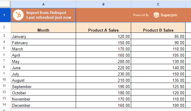
Google Sheets has become an essential tool for organizing and analyzing data, whether for personal use, academic work, or business. However, as your spreadsheet grows, navigating it can become cumbersome.
One common challenge is losing sight of your header row when scrolling through long sheets of data. Understanding how to freeze a row in Sheets can make your workflow more efficient, ensuring that key information is always within view. In this post, we’ll explore different ways to freeze rows in Google Sheets, empowering you to manage your data with ease.
Why Freezing Rows Matters
When working with extensive spreadsheets, especially those containing multiple columns of data, keeping the header row or other crucial information visible is vital. Without it, you may find yourself scrolling back and forth to remember which column corresponds to which data set. This issue is easily solved by learning how to freeze a row in Sheets. Freezing a row allows you to keep certain rows static at the top of your sheet while scrolling through the rest of your data.
Methods to Freeze a Row in Google Sheets
When working with large datasets in Google Sheets, keeping specific rows visible while scrolling can significantly improve your efficiency. Below are four methods to help you freeze a row in Sheets, depending on your preference and the device you're using.
Method 1: Using the View Menu
The most straightforward way to freeze a row in Google Sheets is by using the "View" menu.
Open your Google Sheet: Start by opening the spreadsheet where you want to freeze rows.
Select the row: Click on the row number you wish to freeze. For example, if you want to freeze the top row, click on row 1.
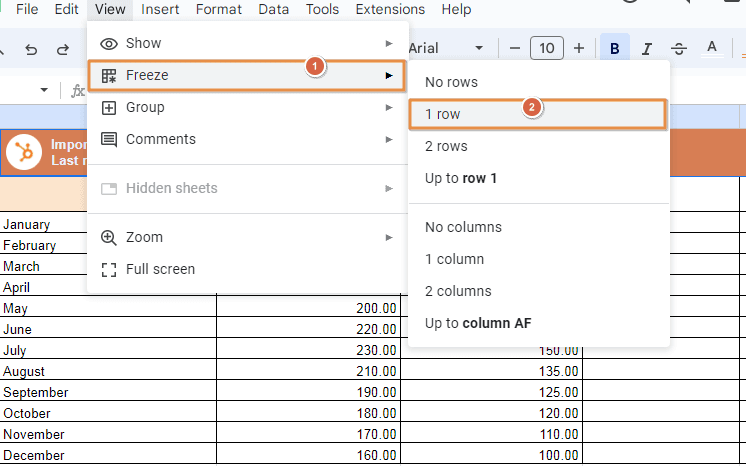
Access the View menu: Navigate to the top of the screen and click on "View".
Freeze the row: Hover over "Freeze" in the dropdown menu, and you'll see options to freeze rows or columns. Click on "1 row" if you selected row 1.
That’s it! You’ve now learned how to freeze a row in Sheets using the View menu. The selected row will stay visible as you scroll through the rest of your data.
If you need to customize your view further or adjust other aspects of your spreadsheet, these methods can help streamline your workflow.
Method 2: Dragging the Freeze Line
Another intuitive way to freeze a row in Google Sheets is by dragging the freeze line directly from the sheet.
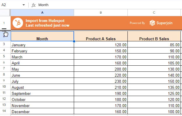
Locate the freeze line: Open your Google Sheet and look at the top left corner where the rows and columns meet. You'll see a thick grey line.
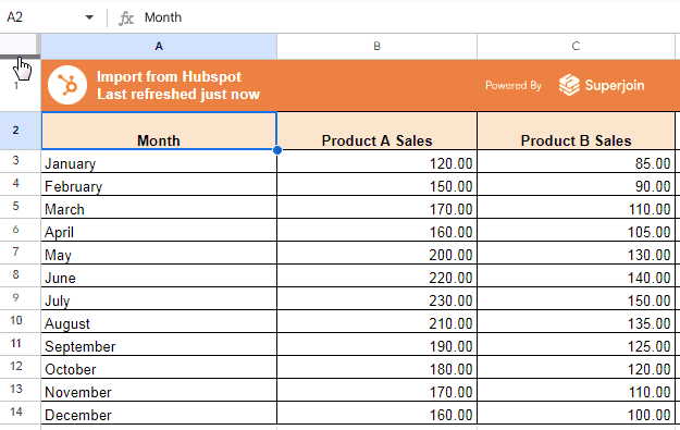
Drag the line down: Click and drag the grey line down to cover the row(s) you want to freeze. For instance, dragging it to cover the first row will freeze only that row.
Confirm the freeze: Once you release the line, the selected row(s) will remain static as you scroll down.
Method 3: Freezing Rows on Mobile
Google Sheets is also accessible on mobile devices, and you can freeze rows directly from your smartphone or tablet.
Open the app: Launch the Google Sheets app on your mobile device and open your spreadsheet.
Tap on the Sheet Name: Tap on the Sheet name, a drop-down menu will appear.
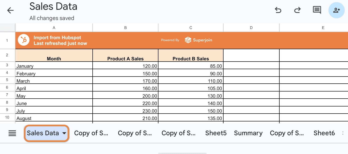
Freeze the row: From the dropdown menu, scroll down and change rows from 0 to 1(or your desired number).

This method is especially handy when you’re on the go and need to quickly lock a row in Google Sheets.
Customizing Your Freeze
Freezing rows in Google Sheets isn’t limited to just the top row. You can freeze multiple rows or even columns to keep them visible as you scroll through your data. This flexibility is useful if you often need to create custom reports or manage different types of data views.
How to Unfreeze All Rows and Columns in Google Sheets
If you've frozen multiple rows or columns and no longer need them to stay in place, unfreezing them is quick and easy. Here’s how you can unfreeze all rows and columns in Google Sheets:
Open your Google Sheet: Start by opening the spreadsheet where rows or columns are frozen.
Go to the View menu: Click on "View" in the top menu.
Unfreeze rows: Hover over the "Freeze" option in the dropdown menu. Then, click on "No rows" to unfreeze all the rows.
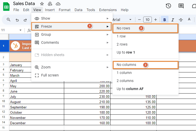
Unfreeze columns: Next, hover over the "Freeze" option again, and click on "No columns" to unfreeze all the columns.
Potential Issues and Troubleshooting
While freezing rows is generally straightforward, there are a few issues you might encounter:
Accidentally freezing too many rows: If you find that more rows are frozen than you intended, you can easily unfreeze them by going to the "View" menu, selecting "Freeze," and choosing "No rows".
Frozen rows not appearing: If you can’t see your frozen row, ensure that you’re scrolling within the correct range. Sometimes, especially in large sheets, it’s easy to lose track of your position.
Conclusion
Learning how to freeze a row in Sheets is a simple yet powerful way to improve your data management. By keeping essential rows visible, you can work more efficiently and reduce errors. Whether you’re using the View menu, dragging the freeze line, or employing keyboard shortcuts, the flexibility offered by Google Sheets makes it easy to customize your experience. Mastering this skill ensures that you’ll never lose track of critical information, no matter how large your spreadsheet grows.
By implementing these methods, you can streamline your workflow, stay organized, and make the most of your Google Sheets experience. If you're dealing with large data sets, check out our tips on automating sales forecasting with Google Sheets to save even more time.
Say Goodbye to Tedious Data Exports! 🚀
Are you tired of the hassle of manually moving data from various tools into Google Sheets? Superjoin has a solution for you.
Superjoin is a Google Sheets add-on that automatically connects your favorite SaaS tools to your spreadsheets. It pulls data directly into Google Sheets, allowing you to create reports that update themselves without any manual work on your part.
Google Sheets has become an essential tool for organizing and analyzing data, whether for personal use, academic work, or business. However, as your spreadsheet grows, navigating it can become cumbersome.
One common challenge is losing sight of your header row when scrolling through long sheets of data. Understanding how to freeze a row in Sheets can make your workflow more efficient, ensuring that key information is always within view. In this post, we’ll explore different ways to freeze rows in Google Sheets, empowering you to manage your data with ease.
Why Freezing Rows Matters
When working with extensive spreadsheets, especially those containing multiple columns of data, keeping the header row or other crucial information visible is vital. Without it, you may find yourself scrolling back and forth to remember which column corresponds to which data set. This issue is easily solved by learning how to freeze a row in Sheets. Freezing a row allows you to keep certain rows static at the top of your sheet while scrolling through the rest of your data.
Methods to Freeze a Row in Google Sheets
When working with large datasets in Google Sheets, keeping specific rows visible while scrolling can significantly improve your efficiency. Below are four methods to help you freeze a row in Sheets, depending on your preference and the device you're using.
Method 1: Using the View Menu
The most straightforward way to freeze a row in Google Sheets is by using the "View" menu.
Open your Google Sheet: Start by opening the spreadsheet where you want to freeze rows.
Select the row: Click on the row number you wish to freeze. For example, if you want to freeze the top row, click on row 1.
Access the View menu: Navigate to the top of the screen and click on "View".
Freeze the row: Hover over "Freeze" in the dropdown menu, and you'll see options to freeze rows or columns. Click on "1 row" if you selected row 1.
That’s it! You’ve now learned how to freeze a row in Sheets using the View menu. The selected row will stay visible as you scroll through the rest of your data.
If you need to customize your view further or adjust other aspects of your spreadsheet, these methods can help streamline your workflow.
Method 2: Dragging the Freeze Line
Another intuitive way to freeze a row in Google Sheets is by dragging the freeze line directly from the sheet.
Locate the freeze line: Open your Google Sheet and look at the top left corner where the rows and columns meet. You'll see a thick grey line.
Drag the line down: Click and drag the grey line down to cover the row(s) you want to freeze. For instance, dragging it to cover the first row will freeze only that row.
Confirm the freeze: Once you release the line, the selected row(s) will remain static as you scroll down.
Method 3: Freezing Rows on Mobile
Google Sheets is also accessible on mobile devices, and you can freeze rows directly from your smartphone or tablet.
Open the app: Launch the Google Sheets app on your mobile device and open your spreadsheet.
Tap on the Sheet Name: Tap on the Sheet name, a drop-down menu will appear.
Freeze the row: From the dropdown menu, scroll down and change rows from 0 to 1(or your desired number).
This method is especially handy when you’re on the go and need to quickly lock a row in Google Sheets.
Customizing Your Freeze
Freezing rows in Google Sheets isn’t limited to just the top row. You can freeze multiple rows or even columns to keep them visible as you scroll through your data. This flexibility is useful if you often need to create custom reports or manage different types of data views.
How to Unfreeze All Rows and Columns in Google Sheets
If you've frozen multiple rows or columns and no longer need them to stay in place, unfreezing them is quick and easy. Here’s how you can unfreeze all rows and columns in Google Sheets:
Open your Google Sheet: Start by opening the spreadsheet where rows or columns are frozen.
Go to the View menu: Click on "View" in the top menu.
Unfreeze rows: Hover over the "Freeze" option in the dropdown menu. Then, click on "No rows" to unfreeze all the rows.
Unfreeze columns: Next, hover over the "Freeze" option again, and click on "No columns" to unfreeze all the columns.
Potential Issues and Troubleshooting
While freezing rows is generally straightforward, there are a few issues you might encounter:
Accidentally freezing too many rows: If you find that more rows are frozen than you intended, you can easily unfreeze them by going to the "View" menu, selecting "Freeze," and choosing "No rows".
Frozen rows not appearing: If you can’t see your frozen row, ensure that you’re scrolling within the correct range. Sometimes, especially in large sheets, it’s easy to lose track of your position.
Conclusion
Learning how to freeze a row in Sheets is a simple yet powerful way to improve your data management. By keeping essential rows visible, you can work more efficiently and reduce errors. Whether you’re using the View menu, dragging the freeze line, or employing keyboard shortcuts, the flexibility offered by Google Sheets makes it easy to customize your experience. Mastering this skill ensures that you’ll never lose track of critical information, no matter how large your spreadsheet grows.
By implementing these methods, you can streamline your workflow, stay organized, and make the most of your Google Sheets experience. If you're dealing with large data sets, check out our tips on automating sales forecasting with Google Sheets to save even more time.
Say Goodbye to Tedious Data Exports! 🚀
Are you tired of the hassle of manually moving data from various tools into Google Sheets? Superjoin has a solution for you.
Superjoin is a Google Sheets add-on that automatically connects your favorite SaaS tools to your spreadsheets. It pulls data directly into Google Sheets, allowing you to create reports that update themselves without any manual work on your part.
FAQs
Can I freeze both rows and columns at the same time in Google Sheets?
Can I freeze both rows and columns at the same time in Google Sheets?
What happens if I freeze a row or column and then delete it?
What happens if I freeze a row or column and then delete it?
Is there a limit to how many rows I can freeze?
Is there a limit to how many rows I can freeze?
Automatic Data Pulls
Visual Data Preview
Set Alerts
other related blogs
Try it now