Google Sheets Tutorial
How To Refresh a Pivot Table in Google Sheets
Exhausted from all the outdated data in your Google Sheets? Get to learn the quick tips and tricks on how to refresh a pivot table in google sheets.
Here's a quick step-by-step guide 🔝
Here's a quick step-by-step guide 🔝
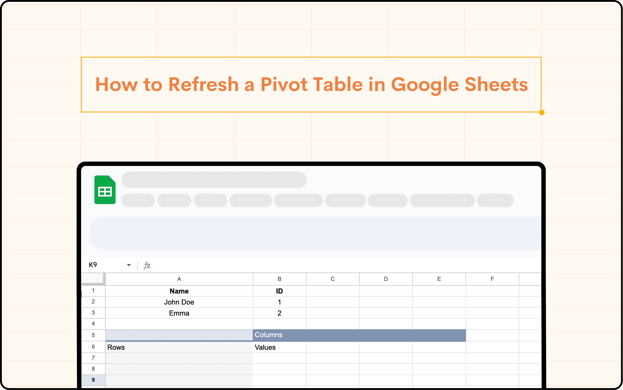


Ever heard of pivot tables? Pivot tables are used when a large dataset is fed into Google Sheets. Sorting and analyzing becomes much easier with pivot tables. If you are still wondering how to refresh a pivot table in Google Sheets, this guide will help you know everything about refreshing the pivot table in Google Sheets with complete data accuracy.
Refresh a Pivot Table in Google Sheets
A pivot table in Google Sheets represents the summary and analysis of the large set of data in the sheets. Even after the data changes, it should reflect in the sheets, and that is when pivot table refresh is used!
How to Create a Pivot Table in Google Sheets?
Pivot tables are simple data in rows and columns that give accurate reports. The powerful pivot table can be created easily in Google Sheets. All you have to do is follow the below steps:
For example,
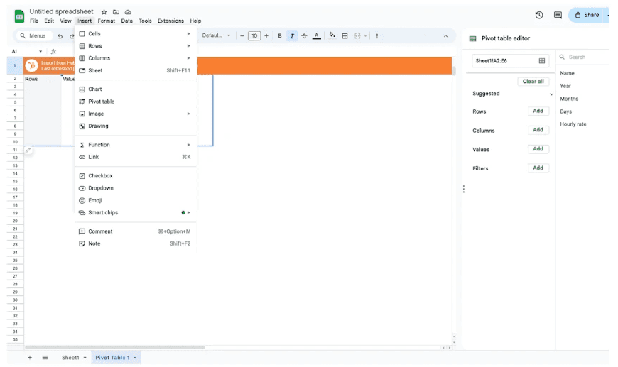
Choose the cells that have the data, click on Insert, and choose Pivot table.
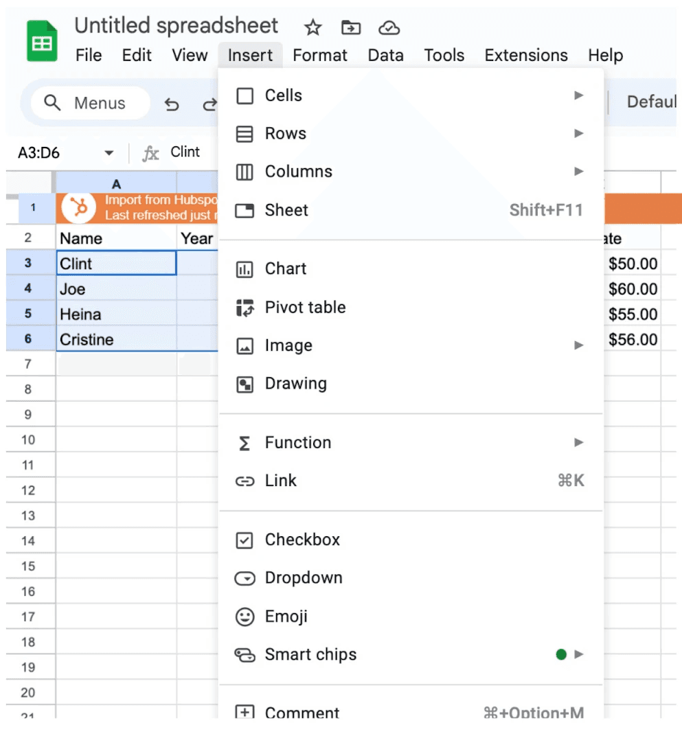
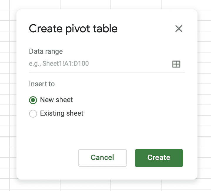
Now, you will see an option to create a pivot table. Click on that and choose “Create”
A table will be populated.
Additionally, you can also export datasets directly from HubSpot into Google Sheets, allowing for seamless integration of your marketing and sales data into your analysis.
Automatic Refresh of a Pivot Table in Google Sheets
For people who wish things were automated and made easier, Google Sheets handles this automatically. Google Sheets has the ability to detect changes made in data or content, and it immediately reflects these changes in the pivot table.
However, for “running” functions like RAND(), TODAY(), NOW(), or custom formulas that depend on time or other changing conditions, one may need to resort to app scripts or extensions for a more dynamic update process. This way, you can always make sure the data is up to date, without any manual intervention.
These methods not only give you updated data but also accurate data as a result.
The Manual Refresh of a Pivot Table in Google Sheets
If your pivot table isn't automatically refreshed, you could use the following methods to refresh it manually.
Method 1: Using the Right-Click Context Menu
If your pivot table isn’t refreshing automatically, it might be because some rows or columns are outside the data range. Here’s how to fix it:
At the bottom left corner of the Pivot table click on the edit option to open the Pivot table editor.
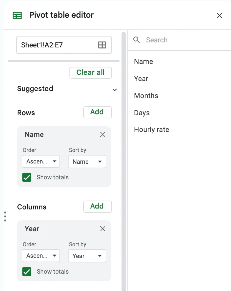
Choose the data range box in the Pivot table editor
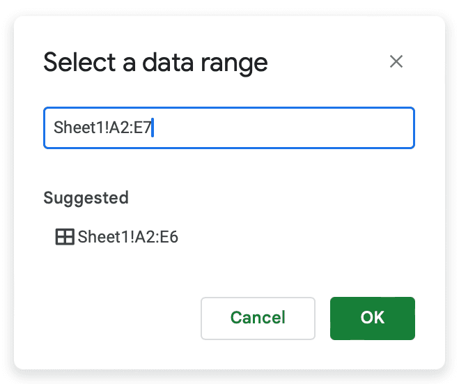
You can refresh the data by editing the rows and columns here
Method 2: Keyboard Shortcut
If your pivot table isn’t refreshing automatically, you can manually refresh the current page to ensure your data is up-to-date. Here’s how you can do it with a keyboard shortcut:
On your Mac, press Command + Shift + F5
On your Windows/Linux, Press Ctrl + Shift + F5.

Tips and Tricks to Remember While Refreshing a Pivot Table in Google Sheets
There are certain tips and tricks that must be remembered for a better understanding and usage of the pivot tables in Google Sheets.
To Speed Up the Process: Use the F5 key to refresh instantly to make changes to the original data.
To maintain accuracy: Under “Source data”, you can double check if the new data is entered in the pivot table. You can also remove filters applied on the pivot table, to prevent any changes made in the source data.
Additional Points to be Noted
Identify the Pivot Table Cell: Do you know that clicking anywhere within the pivot table can refresh it? Yes! It is not necessary to select the entire table for it.
Have alternate options: If you are performing just minor actions on the pivot table, a refresh might not be necessary every time you do this. All you have to do is simply scroll through the table to see if the updated data is present or not.
By keeping these points in mind, your pivot table refresh becomes easy and your data will be updated!
Common Mistakes to be Avoided
Refreshing a pivot table can be easier when heard, but sometimes, people tend to make common mistakes. To avoid these encounters, here are some useful pointers:
Always select the entire data range to avoid incomplete results when the pivot table is refreshed.
Refresh after any date changes are made, either manually or automatically.
Work on the errors and warnings.
Review the pivot table layout and formatting.
Mistakes are commonly made. When avoided with proactive steps, a perfect and updated pivot table will be in front of your eyes!
Thinking of choosing a good platform to get all these done automatically? Superjoin is here to help you out! Reach out to Superjoin, book your calendars with us and schedule a demo for a live session! We are here to deliver the difference!
Ever heard of pivot tables? Pivot tables are used when a large dataset is fed into Google Sheets. Sorting and analyzing becomes much easier with pivot tables. If you are still wondering how to refresh a pivot table in Google Sheets, this guide will help you know everything about refreshing the pivot table in Google Sheets with complete data accuracy.
Refresh a Pivot Table in Google Sheets
A pivot table in Google Sheets represents the summary and analysis of the large set of data in the sheets. Even after the data changes, it should reflect in the sheets, and that is when pivot table refresh is used!
How to Create a Pivot Table in Google Sheets?
Pivot tables are simple data in rows and columns that give accurate reports. The powerful pivot table can be created easily in Google Sheets. All you have to do is follow the below steps:
For example,
Choose the cells that have the data, click on Insert, and choose Pivot table.

Now, you will see an option to create a pivot table. Click on that and choose “Create”

A table will be populated.
Additionally, you can also export datasets directly from HubSpot into Google Sheets, allowing for seamless integration of your marketing and sales data into your analysis.

Automatic Refresh of a Pivot Table in Google Sheets
For people who wish things were automated and made easier, Google Sheets handles this automatically. Google Sheets has the ability to detect changes made in data or content, and it immediately reflects these changes in the pivot table.
However, for “running” functions like RAND(), TODAY(), NOW(), or custom formulas that depend on time or other changing conditions, one may need to resort to app scripts or extensions for a more dynamic update process. This way, you can always make sure the data is up to date, without any manual intervention.
These methods not only give you updated data but also accurate data as a result.
The Manual Refresh of a Pivot Table in Google Sheets
If your pivot table isn't automatically refreshed, you could use the following methods to refresh it manually.
Method 1: Using the Right-Click Context Menu
If your pivot table isn’t refreshing automatically, it might be because some rows or columns are outside the data range. Here’s how to fix it:
At the bottom left corner of the Pivot table click on the edit option to open the Pivot table editor.

Choose the data range box in the Pivot table editor

You can refresh the data by editing the rows and columns here
Method 2: Keyboard Shortcut
If your pivot table isn’t refreshing automatically, you can manually refresh the current page to ensure your data is up-to-date. Here’s how you can do it with a keyboard shortcut:
On your Mac, press Command + Shift + F5
On your Windows/Linux, Press Ctrl + Shift + F5.

Tips and Tricks to Remember While Refreshing a Pivot Table in Google Sheets
There are certain tips and tricks that must be remembered for a better understanding and usage of the pivot tables in Google Sheets.
To Speed Up the Process: Use the F5 key to refresh instantly to make changes to the original data.
To maintain accuracy: Under “Source data”, you can double check if the new data is entered in the pivot table. You can also remove filters applied on the pivot table, to prevent any changes made in the source data.
Additional Points to be Noted
Identify the Pivot Table Cell: Do you know that clicking anywhere within the pivot table can refresh it? Yes! It is not necessary to select the entire table for it.
Have alternate options: If you are performing just minor actions on the pivot table, a refresh might not be necessary every time you do this. All you have to do is simply scroll through the table to see if the updated data is present or not.
By keeping these points in mind, your pivot table refresh becomes easy and your data will be updated!
Common Mistakes to be Avoided
Refreshing a pivot table can be easier when heard, but sometimes, people tend to make common mistakes. To avoid these encounters, here are some useful pointers:
Always select the entire data range to avoid incomplete results when the pivot table is refreshed.
Refresh after any date changes are made, either manually or automatically.
Work on the errors and warnings.
Review the pivot table layout and formatting.
Mistakes are commonly made. When avoided with proactive steps, a perfect and updated pivot table will be in front of your eyes!
Thinking of choosing a good platform to get all these done automatically? Superjoin is here to help you out! Reach out to Superjoin, book your calendars with us and schedule a demo for a live session! We are here to deliver the difference!
FAQs
How often should I refresh my pivot table?
How often should I refresh my pivot table?
Why is my pivot table not updating after I refresh it?
Why is my pivot table not updating after I refresh it?
Can we refresh multiple pivot tables simultaneously?
Can we refresh multiple pivot tables simultaneously?
Automatic Data Pulls
Visual Data Preview
Set Alerts
other related blogs
Try it now
