Microsoft Excel Tutorial
How to Freeze a Row in Microsoft Excel
Learn how to freeze a row in Excel to keep your headers visible while scrolling. Various methods for freezing or locking rows in Excel.
Table of Contents
Excel has developed into a vital tool for data organization and analysis, whether for corporate, academic, or personal use. But if your spreadsheet gets bigger, it can be difficult to navigate.
When scrolling through lengthy data sheets, one common problem is losing sight of your header row. Your workflow will be more effective if you know how to freeze a row in Excel so that important data is always visible. We'll look at many methods for freezing rows in Excel in this post so you can easily manage your data.
Why Freezing Rows Matters
It's critical to maintain the header row and other important information visible when dealing with large spreadsheets, particularly those with several data fields. If you don't have it, you might have to go back and forth to remember which data set goes with which column. By knowing how to freeze a row in Excel, this problem can be resolved with ease. You can scroll through the rest of your data while keeping some rows at the top of your sheet static by freezing a row.
Methods to Freeze a Row in Excel
When working with large datasets in Excel, keeping specific rows visible while scrolling can significantly improve your efficiency. Below are four methods to help you freeze a row in Sheets, depending on your preference and the device you're using.
Method 1: Using the View Menu
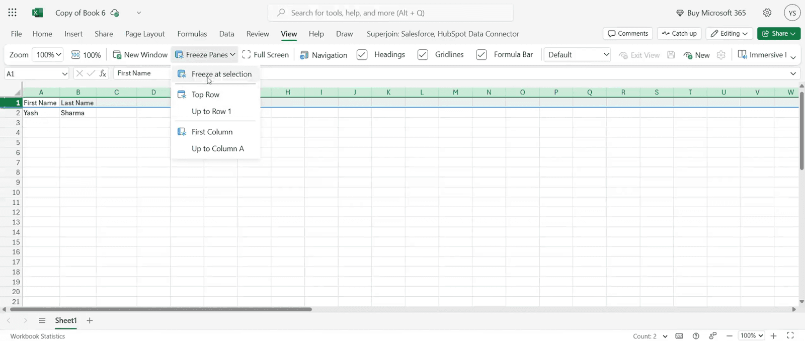
The most straightforward way to freeze a row in Excel is by using the "View" menu.
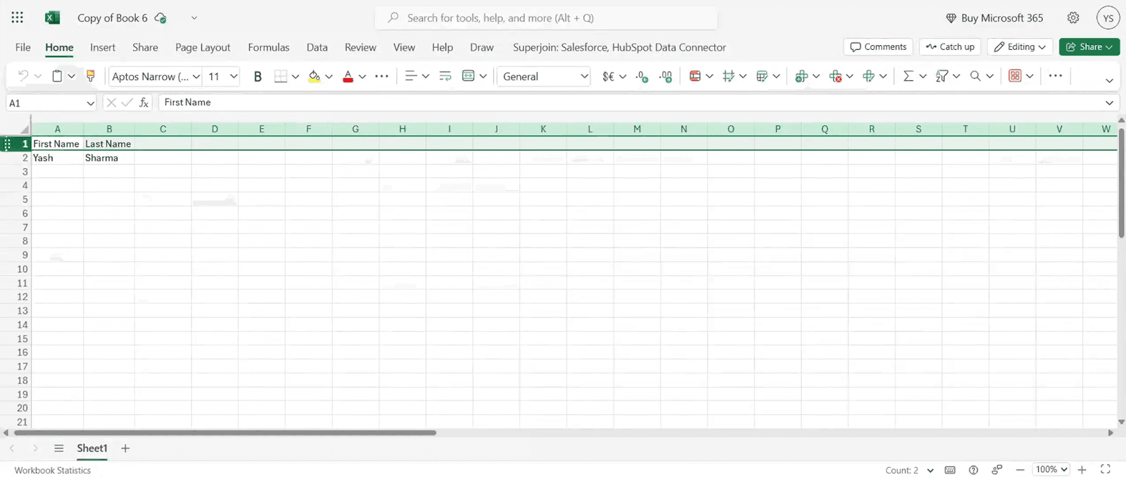
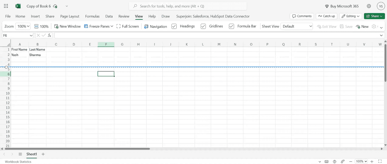
To lock a row, first select the row you wish to freeze
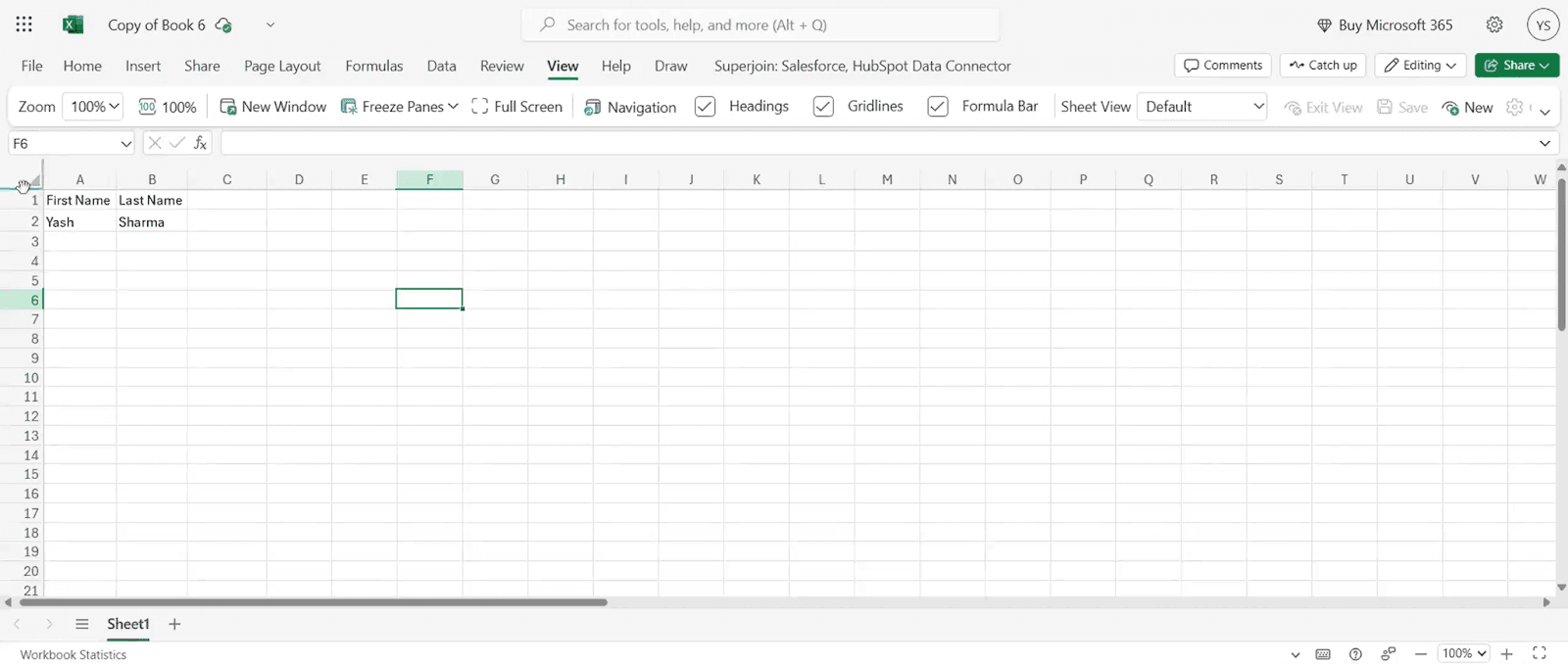
Next, navigate to the View tab, click on Freeze Panes, and then select Freeze at Selection. This action will lock the row you have selected.
That's it! Now you know how to use the View option in Excel to freeze a row. As you scroll through the remainder of your data, the selected row will remain visible.
Method 2: Dragging the Freeze Line
Locate the freeze line: Examine the upper left corner of your Excel sheet, where the rows and columns converge. A thick grey line will be visible.
Drag it to whichever column or row you wish to freeze. Simply drag it until you reach the row or column you want to freeze, then release it. This action will ensure that the selected rows or columns remain visible at all times while you navigate through your worksheet.
Customizing Your Freeze
Excel allows you to freeze rows other than the top row. To maintain visibility while you browse through your data, you can freeze a number of rows or even columns. If you frequently need to manage various data view types or build bespoke reports, this flexibility is helpful.
How to Unfreeze All Rows and Columns in Excel
To unfreeze the row, again select the entire row, go to the View tab, click on Freeze Panes, and choose the Unfreeze option.
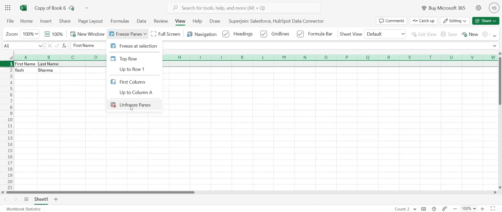
All the rows are now unfreezed.
Potential Issues and Troubleshooting
Although freezing rows is usually simple, you may run into the following problems:
Unintentionally freezing too many rows: Access the "View" menu, pick "Freeze," and then select "No rows" to quickly unfreeze any rows that have been accidentally frozen.
Frozen rows not showing up: Make sure you're scrolling inside the appropriate range if your frozen row is not visible. It might be simple to lose sight of your position at times, particularly when working with huge sheets.
Conclusion
A straightforward yet effective method to enhance your data management is to learn how to freeze a row in Excel. You can increase productivity and decrease errors by keeping important rows visible. Excel's versatility makes it simple to personalize your experience, whether you're using the View menu, dragging the freeze line, or using keyboard shortcuts. Gaining proficiency in this area will guarantee that, regardless of how big your spreadsheet gets, you never lose sight of important data.
You can maximize your Excel experience, maintain organization, and expedite your productivity by putting these strategies into practice. To save even more time when working with massive data sets, see our advice on using Excel to automate sales forecasting.
Say Goodbye to Tedious Data Exports! 🚀
Are you tired of the hassle of manually moving data from various tools into Excel? Superjoin has a solution for you.
Superjoin is an Excel add-in that automatically connects your favorite SaaS tools to your spreadsheets. It pulls data directly into Excel, allowing you to create reports that update themselves without any manual work on your part.
Bid farewell to tedious exports and repetitive tasks. With Superjoin, you can add one additional day to your week. Try Superjoin for free or schedule a demo.
Excel has developed into a vital tool for data organization and analysis, whether for corporate, academic, or personal use. But if your spreadsheet gets bigger, it can be difficult to navigate.
When scrolling through lengthy data sheets, one common problem is losing sight of your header row. Your workflow will be more effective if you know how to freeze a row in Excel so that important data is always visible. We'll look at many methods for freezing rows in Excel in this post so you can easily manage your data.
Why Freezing Rows Matters
It's critical to maintain the header row and other important information visible when dealing with large spreadsheets, particularly those with several data fields. If you don't have it, you might have to go back and forth to remember which data set goes with which column. By knowing how to freeze a row in Excel, this problem can be resolved with ease. You can scroll through the rest of your data while keeping some rows at the top of your sheet static by freezing a row.
Methods to Freeze a Row in Excel
When working with large datasets in Excel, keeping specific rows visible while scrolling can significantly improve your efficiency. Below are four methods to help you freeze a row in Sheets, depending on your preference and the device you're using.
Method 1: Using the View Menu
The most straightforward way to freeze a row in Excel is by using the "View" menu.
To lock a row, first select the row you wish to freeze
Next, navigate to the View tab, click on Freeze Panes, and then select Freeze at Selection. This action will lock the row you have selected.
That's it! Now you know how to use the View option in Excel to freeze a row. As you scroll through the remainder of your data, the selected row will remain visible.
Method 2: Dragging the Freeze Line
Locate the freeze line: Examine the upper left corner of your Excel sheet, where the rows and columns converge. A thick grey line will be visible.
Drag it to whichever column or row you wish to freeze. Simply drag it until you reach the row or column you want to freeze, then release it. This action will ensure that the selected rows or columns remain visible at all times while you navigate through your worksheet.
Customizing Your Freeze
Excel allows you to freeze rows other than the top row. To maintain visibility while you browse through your data, you can freeze a number of rows or even columns. If you frequently need to manage various data view types or build bespoke reports, this flexibility is helpful.
How to Unfreeze All Rows and Columns in Excel
To unfreeze the row, again select the entire row, go to the View tab, click on Freeze Panes, and choose the Unfreeze option.
All the rows are now unfreezed.
Potential Issues and Troubleshooting
Although freezing rows is usually simple, you may run into the following problems:
Unintentionally freezing too many rows: Access the "View" menu, pick "Freeze," and then select "No rows" to quickly unfreeze any rows that have been accidentally frozen.
Frozen rows not showing up: Make sure you're scrolling inside the appropriate range if your frozen row is not visible. It might be simple to lose sight of your position at times, particularly when working with huge sheets.
Conclusion
A straightforward yet effective method to enhance your data management is to learn how to freeze a row in Excel. You can increase productivity and decrease errors by keeping important rows visible. Excel's versatility makes it simple to personalize your experience, whether you're using the View menu, dragging the freeze line, or using keyboard shortcuts. Gaining proficiency in this area will guarantee that, regardless of how big your spreadsheet gets, you never lose sight of important data.
You can maximize your Excel experience, maintain organization, and expedite your productivity by putting these strategies into practice. To save even more time when working with massive data sets, see our advice on using Excel to automate sales forecasting.
Say Goodbye to Tedious Data Exports! 🚀
Are you tired of the hassle of manually moving data from various tools into Excel? Superjoin has a solution for you.
Superjoin is an Excel add-in that automatically connects your favorite SaaS tools to your spreadsheets. It pulls data directly into Excel, allowing you to create reports that update themselves without any manual work on your part.
Bid farewell to tedious exports and repetitive tasks. With Superjoin, you can add one additional day to your week. Try Superjoin for free or schedule a demo.
FAQs
Can I freeze both rows and columns at the same time in Excel?
Can I freeze both rows and columns at the same time in Excel?
What happens if I freeze a row or column and then delete it?
What happens if I freeze a row or column and then delete it?
Is there a limit to how many rows I can freeze?
Is there a limit to how many rows I can freeze?
Automatic Data Pulls
Visual Data Preview
Set Alerts
other related blogs

Try it now